Statistical Thinking using Randomisation and Simulation
Compiling data for problem solving
Di Cook (dicook@monash.edu, @visnut)
W10.C1
Overview of this class
- What is
tidy data? Why do you want tidy data? Getting your data into tidy form using tidyr. - Wrangling verbs:
filter,arrange,select,mutate,summarise, with dplyr - Date and time with lubridate
Terminology
Cases, records, individuals, subjects, experimental units, example, instance: things we are collecting information aboutVariables, attributes, fields, features: what we are measuring on each record/case/.../instance
Generally we think of cases being on the rows, and variables being in the columns of a table. This is a basic data structure. BUT data often is given to us in many other shapes than this. Getting into a tidy shape will allow you to efficiently use it for modeling.
Example 1
#> # A tibble: 4 x 4#> Inst AvNumPubs AvNumCits PctCompletion#> <chr> <dbl> <dbl> <dbl>#> 1 ARIZONA STATE UNIVERSITY 0.90 1.57 31.7#> 2 AUBURN UNIVERSITY 0.79 0.64 44.4#> 3 BOSTON COLLEGE 0.51 1.03 46.8#> 4 BOSTON UNIVERSITY 0.49 2.66 34.2- Cases: __
- Variables: __
Example 2
Data from weather stations available at NCDC NOAA
#> V1 V2 V3 V4 V5 V9 V13 V17 V21 V25 V29 V33 V37 V41 V45 V49#> 1 ASN00086282 1970 7 TMAX 141 124 113 123 148 149 139 153 123 108 119 112#> 2 ASN00086282 1970 7 TMIN 80 63 36 57 69 47 84 78 49 42 48 56#> 3 ASN00086282 1970 7 PRCP 3 30 0 0 36 3 0 0 10 23 3 0#> 4 ASN00086282 1970 8 TMAX 145 128 150 122 109 112 116 142 166 127 117 127#> V53 V57 V61 V65 V69 V73 V77 V81 V85 V89 V93 V97 V101 V105 V109 V113 V117#> 1 126 112 115 133 134 126 104 143 141 134 117 142 158 149 133 143 150#> 2 51 36 44 39 40 58 15 33 51 74 39 66 78 36 61 46 42#> 3 5 0 0 0 0 0 8 0 18 0 0 0 0 13 3 0 25#> 4 159 143 114 65 113 125 129 147 161 168 178 161 145 142 137 150 120#> V121 V125#> 1 145 115#> 2 63 39#> 3 0 3#> 4 114 129- Cases: __
- Variables: __
Example 3
Here are the column headers from a data set containing information on tuberculosis incidence by country across the globe for the last few decades ...
#> [1] "iso2" "year" "m_04" "m_514" "m_014" "m_1524" "m_2534"#> [8] "m_3544" "m_4554" "m_5564" "m_65" "m_u" "f_04" "f_514" #> [15] "f_014" "f_1524" "f_2534" "f_3544" "f_4554" "f_5564" "f_65" #> [22] "f_u"- Cases: __
- Variables: __
Example 4
We'll commonly find these data on web sites:
#> religion <$10k $10-20k $20-30k $30-40k#> 1 Agnostic 27 34 60 81#> 2 Atheist 12 27 37 52#> 3 Buddhist 27 21 30 34#> 4 Catholic 418 617 732 670#> 5 Don’t know/refused 15 14 15 11- Cases: __
- Variables: __
Example 5
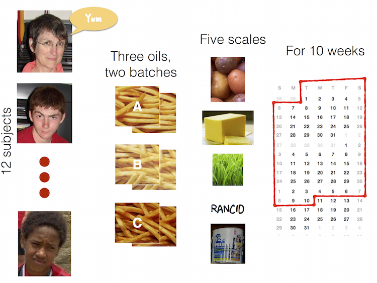
10 week sensory experiment, 12 individuals assessed taste of french fries on several scales (how potato-y, buttery, grassy, rancid, paint-y do they taste?), fried in one of 3 different oils, replicated twice. First few rows:
| time | treatment | subject | rep | potato | buttery | grassy | rancid | painty |
|---|---|---|---|---|---|---|---|---|
| 1 | 1 | 3 | 1 | 2.9 | 0.0 | 0.0 | 0.0 | 5.5 |
| 1 | 1 | 3 | 2 | 14.0 | 0.0 | 0.0 | 1.1 | 0.0 |
| 1 | 1 | 10 | 1 | 11.0 | 6.4 | 0.0 | 0.0 | 0.0 |
| 1 | 1 | 10 | 2 | 9.9 | 5.9 | 2.9 | 2.2 | 0.0 |
What do you like to know?
Messy data patterns
There are various features of messy data that one can observe in practice. Here are some of the more commonly observed patterns.
- Column headers are values, not variable names
- Variables are stored in both rows and columns, contingency table format
- Information stored in multiple tables
- Dates in many different formats
- Not easy to analyse
What is tidy data?
- Each observation forms a row
- Each variable forms a column
- Contained in a single table
- Long form makes it easier to reshape in many different ways
- Wide form is common for analysis/modeling
- This form neatly fits into the statistical thinking framework, where you can anticipate the variables being a sample from some statistical distribution.
Tidy vs messy
- Tidy data facilitates analysis in many different ways, answering multiple questions, applying methods to new data or other problems
- Messy data may work for one particular problem but is not generalisable
Tidy verbs
gather: specify thekeys(identifiers) and thevalues(measures) to make long form (used to be called melting)spread: variables in columns (used to be called casting)nest/unnest: working with listsseparate/unite: split and combine columns
French fries example
#> time treatment subject rep potato buttery grassy rancid painty#> 61 1 1 3 1 2.9 0.0 0.0 0.0 5.5#> 25 1 1 3 2 14.0 0.0 0.0 1.1 0.0#> 62 1 1 10 1 11.0 6.4 0.0 0.0 0.0#> 26 1 1 10 2 9.9 5.9 2.9 2.2 0.0#> 63 1 1 15 1 1.2 0.1 0.0 1.1 5.1#> 27 1 1 15 2 8.8 3.0 3.6 1.5 2.3This format is not ideal for data analysis
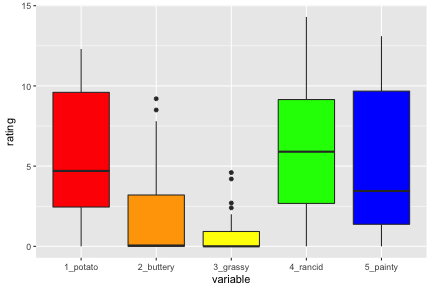
What code would be needed to plot each of the ratings over time as a different color?
library(ggplot2)french_sub <- french_fries[french_fries$time == 10,]ggplot(data = french_sub) + geom_boxplot(aes(x="1_potato", y=potato), fill = I("red")) + geom_boxplot(aes(x = "2_buttery", y = buttery), fill = I("orange")) + geom_boxplot(aes(x = "3_grassy", y = grassy), fill = I("yellow")) + geom_boxplot(aes(x = "4_rancid", y = rancid), fill = I("green")) + geom_boxplot(aes(x = "5_painty", y = painty), fill = I("blue")) + xlab("variable") + ylab("rating")The plot
Wide to long
Gathering
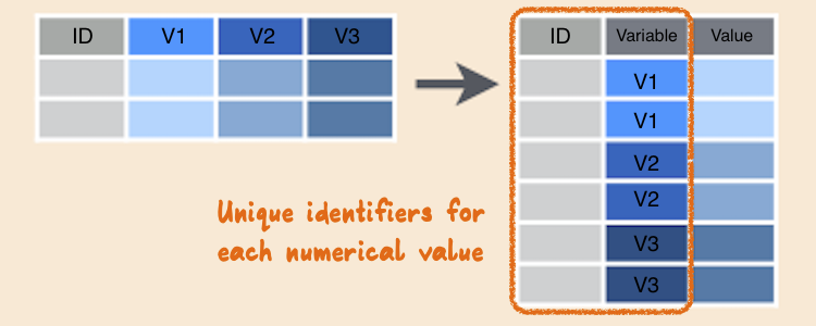
- When gathering, you need to specify the keys (identifiers) and the values (measures).
- Keys/Identifiers:
- Identify a record (must be unique)
- Example: Indices on an random variable
- Fixed by design of experiment (known in advance)
- May be single or composite (may have one or more variables)
- Values/Measures:
- Collected during the experiment (not known in advance)
- Usually numeric quantities
Gathering the French Fries data
ff_long <- gather(french_fries, key = variable, value = rating, potato:painty)head(ff_long)#> time treatment subject rep variable rating#> 1 1 1 3 1 potato 2.9#> 2 1 1 3 2 potato 14.0#> 3 1 1 10 1 potato 11.0#> 4 1 1 10 2 potato 9.9#> 5 1 1 15 1 potato 1.2#> 6 1 1 15 2 potato 8.8Let's re-write the code
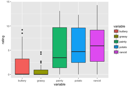
ff_long_sub <- ff_long %>% filter(time == 10)ggplot(data = ff_long_sub, aes(x=variable, y=rating, fill = variable)) + geom_boxplot()And plot it
Long to wide
In certain applications, we may wish to take a long dataset and convert it to a wide dataset (Perhaps displaying in a table).
#> time treatment subject rep variable rating#> 1 1 1 3 1 potato 2.9#> 2 1 1 3 2 potato 14.0#> 3 1 1 10 1 potato 11.0#> 4 1 1 10 2 potato 9.9#> 5 1 1 15 1 potato 1.2#> 6 1 1 15 2 potato 8.8Spread
We use the spread function from tidyr to do this:
ff_wide <- spread(ff_long, key = variable, value = rating)head(ff_wide)#> time treatment subject rep buttery grassy painty potato rancid#> 1 1 1 3 1 0.0 0.0 5.5 2.9 0.0#> 2 1 1 3 2 0.0 0.0 0.0 14.0 1.1#> 3 1 1 10 1 6.4 0.0 0.0 11.0 0.0#> 4 1 1 10 2 5.9 2.9 0.0 9.9 2.2#> 5 1 1 15 1 0.1 0.0 5.1 1.2 1.1#> 6 1 1 15 2 3.0 3.6 2.3 8.8 1.5The split-apply-combine approach
- Split a dataset into many smaller sub-datasets
- Apply some function to each sub-dataset to compute a result
- Combine the results of the function calls into a one dataset
The split-apply-combine approach
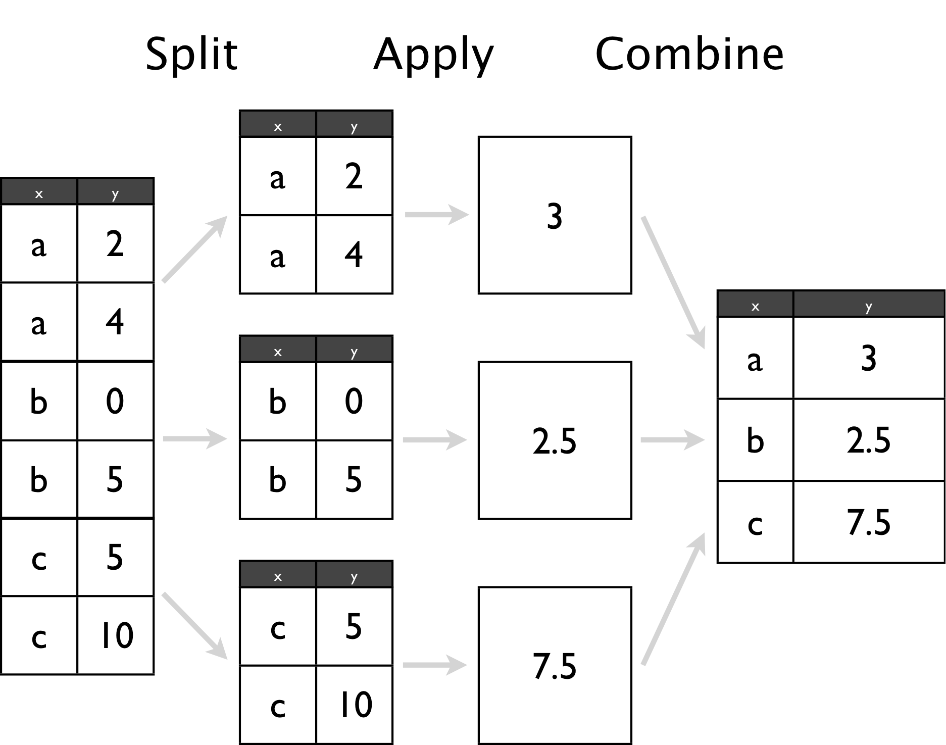
Split-apply-combine in dplyr
library(dplyr)ff_summary <- ff_long %>% group_by(variable) %>% # SPLIT summarise( m = mean(rating, na.rm = TRUE), s=sd(rating, na.rm=TRUE)) # APPLY + COMBINEff_summary#> # A tibble: 5 x 3#> variable m s#> <chr> <dbl> <dbl>#> 1 buttery 1.8236994 2.409758#> 2 grassy 0.6641727 1.320574#> 3 painty 2.5217579 3.393717#> 4 potato 6.9525180 3.584403#> 5 rancid 3.8522302 3.781815Pipes
- Pipes historically enable data analysis pipelines
- Pipes allow the code to be read like a sequence of operations
- dplyr allows us to chain together these data analysis tasks using the
%>%(pipe) operator x %>% f(y)is shorthand forf(x, y)- Example:
student2012.sub <- readRDS("../data/student_sub.rds")student2012.sub %>% count(CNT) #> # A tibble: 43 x 2#> CNT n#> <chr> <int>#> 1 ARE 11500#> 2 AUS 14481#> 3 AUT 4755#> 4 BEL 8597#> 5 BGR 5282#> 6 BRA 5506#> 7 CAN 21544#> 8 CHL 6856#> 9 COL 9073#> 10 CZE 5327#> # ... with 33 more rowsdplyr verbs
There are five primary dplyr verbs, representing distinct data analysis tasks:
Filter: Remove the rows of a data frame, producing subsetsArrange: Reorder the rows of a data frameSelect: Select particular columns of a data frameMutate: Add new columns that are functions of existing columnsSummarise: Create collapsed summaries of a data frame
Filter
french_fries %>% filter(subject == 3, time == 1)#> time treatment subject rep potato buttery grassy rancid painty#> 1 1 1 3 1 2.9 0.0 0.0 0.0 5.5#> 2 1 1 3 2 14.0 0.0 0.0 1.1 0.0#> 3 1 2 3 1 13.9 0.0 0.0 3.9 0.0#> 4 1 2 3 2 13.4 0.1 0.0 1.5 0.0#> 5 1 3 3 1 14.1 0.0 0.0 1.1 0.0#> 6 1 3 3 2 9.5 0.0 0.6 2.8 0.0Arrange
french_fries %>% arrange(desc(rancid)) %>% head#> time treatment subject rep potato buttery grassy rancid painty#> 1 9 2 51 1 7.3 2.3 0 14.9 0.1#> 2 10 1 86 2 0.7 0.0 0 14.3 13.1#> 3 5 2 63 1 4.4 0.0 0 13.8 0.6#> 4 9 2 63 1 1.8 0.0 0 13.7 12.3#> 5 5 2 19 2 5.5 4.7 0 13.4 4.6#> 6 4 3 63 1 5.6 0.0 0 13.3 4.4Select
french_fries %>% select(time, treatment, subject, rep, potato) %>% head#> time treatment subject rep potato#> 61 1 1 3 1 2.9#> 25 1 1 3 2 14.0#> 62 1 1 10 1 11.0#> 26 1 1 10 2 9.9#> 63 1 1 15 1 1.2#> 27 1 1 15 2 8.8Mutate
french_fries %>% mutate(yucky = grassy+rancid+painty) %>% head#> time treatment subject rep potato buttery grassy rancid painty yucky#> 1 1 1 3 1 2.9 0.0 0.0 0.0 5.5 5.5#> 2 1 1 3 2 14.0 0.0 0.0 1.1 0.0 1.1#> 3 1 1 10 1 11.0 6.4 0.0 0.0 0.0 0.0#> 4 1 1 10 2 9.9 5.9 2.9 2.2 0.0 5.1#> 5 1 1 15 1 1.2 0.1 0.0 1.1 5.1 6.2#> 6 1 1 15 2 8.8 3.0 3.6 1.5 2.3 7.4Summarise
french_fries %>% group_by(time, treatment) %>% summarise(mean_rancid = mean(rancid), sd_rancid = sd(rancid))#> # A tibble: 30 x 4#> # Groups: time [?]#> time treatment mean_rancid sd_rancid#> <fctr> <fctr> <dbl> <dbl>#> 1 1 1 2.758333 3.212870#> 2 1 2 1.716667 2.714801#> 3 1 3 2.600000 3.202037#> 4 2 1 3.900000 4.374730#> 5 2 2 2.141667 3.117540#> 6 2 3 2.495833 3.378767#> 7 3 1 4.650000 3.933358#> 8 3 2 2.895833 3.773532#> 9 3 3 3.600000 3.592867#> 10 4 1 2.079167 2.394737#> # ... with 20 more rowsDates and times
- Dates are deceptively hard to work with
- 02/05/2012. Is it February 5th, or May 2nd?
- Time zones
- Different starting times of stock markets, airplane departure and arrival
Basic lubridate use
library(lubridate)now()#> [1] "2017-09-30 15:05:22 AEST"now(tz = "America/Chicago")#> [1] "2017-09-30 00:05:22 CDT"today()#> [1] "2017-09-30"now() + hours(4)#> [1] "2017-09-30 19:05:22 AEST"today() - days(2)#> [1] "2017-09-28"ymd("2013-05-14")#> [1] "2013-05-14"mdy("05/14/2013")#> [1] "2013-05-14"dmy("14052013")#> [1] "2013-05-14"Dates example: Oscars date of birth
oscars <- read_csv("../data/oscars.csv")oscars <- oscars %>% mutate(DOB = mdy(DOB))head(oscars$DOB)#> [1] "1895-09-30" "1884-07-23" "1894-04-23" "2006-10-06" "1886-02-02"#> [6] "1892-04-08"summary(oscars$DOB)#> Min. 1st Qu. Median Mean 3rd Qu. #> "1868-04-10" "1934-09-18" "1957-06-23" "1962-05-21" "2008-04-05" #> Max. #> "2029-12-13"Calculating on dates
- You should never ask a woman her age, but ... really!
oscars <- oscars %>% mutate(year=year(DOB))summary(oscars$year)#> Min. 1st Qu. Median Mean 3rd Qu. Max. #> 1868 1934 1957 1962 2008 2029oscars %>% filter(year == "2029") %>% select(Name, Sex, DOB)#> # A tibble: 4 x 3#> Name Sex DOB#> <chr> <chr> <date>#> 1 Audrey Hepburn Female 2029-05-04#> 2 Grace Kelly Female 2029-11-12#> 3 Miyoshi Umeki Female 2029-04-03#> 4 Christopher Plummer Male 2029-12-13Months
oscars <- oscars %>% mutate(month=month(DOB, label = TRUE, abbr = TRUE))table(oscars$month)#> #> Jan Feb Mar Apr May Jun Jul Aug Sep Oct Nov Dec #> 32 35 37 53 35 27 37 33 31 31 30 42Now plot it
ggplot(data=oscars, aes(month)) + geom_bar()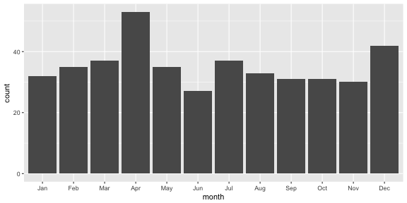
Should you be born in April?
df <- data.frame(m=sample(1:12, 423, replace=TRUE))df$m2 <- factor(df$m, levels=1:12, labels=month.abb)ggplot(data=df, aes(x=m2)) + geom_bar()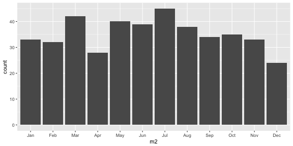
Share and share alike

This work is licensed under a Creative Commons Attribution 4.0 International License.