Statistical Thinking using Randomisation and Simulation
Multilevel Models
Di Cook (dicook@monash.edu, @visnut)
W7.C1
Overview of this class
- Fixed effects vs random effects
- Mixed effects models
- Diagnostics
What is a multilevel model?
- Observations are not independent, but belong to a hierarchy
- Example: individual level demographics (age, gender), and school level information (location, cours offerings, classroom resources)
- Multilevel model enables fitting different types of dependencies
Fixed vs random
Fixed effectscan be used when you know all the categories, e.g. age, gender, smoking statusRandom effectsare used when not all groups are captured, and we have a random selection of the groups, e.g. individuals (if you have multiple measurements), schools, hospitals
Mixed effects models - a type of multilevel model
For data organized in g groups, consider a continuous response linear mixed-effects model (LME model) for each group i, i=1,…,g:
yi(ni×1)=Xi(ni×p)β(p×1)+Zi(ni×q)bi(q×1)+εi(ni×1)
yiis the vector of outcomes for thenilevel-1 units in groupiXiandZiare design matrices for the fixed and random effectsβis a vector ofpfixed effects governing the global mean structurebiis a vector ofqrandom effects for between-group covarianceεiis a vector of level-1 error terms for within-group covariance
Example
- Data:
radon, 919 owner-occupied homes in 85 counties of Minnesota. Available in theHLMdiagpackage - Response:
log.radon - Fixed:
storey(categorical) - Covariate:
uranium(quantitative) - Random:
county(house is a member of county)
## Observations: 919## Variables: 5## $ log.radon <dbl> 0.7885, 0.7885, 1.0647, 0.0000, 1.1314, 0.9163, 0....## $ storey <int> 1, 0, 0, 0, 0, 0, 0, 0, 0, 0, 0, 0, 0, 0, 0, 0, 0,...## $ uranium <dbl> -0.689, -0.689, -0.689, -0.689, -0.847, -0.847, -0...## $ county <int> 1, 1, 1, 1, 2, 2, 2, 2, 2, 2, 2, 2, 2, 2, 2, 2, 2,...## $ county.name <fctr> AITKIN, AITKIN, AITKIN, AITKIN, ANOKA, ANOKA, ANO...Take a look
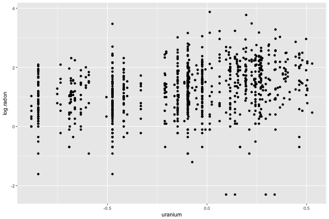
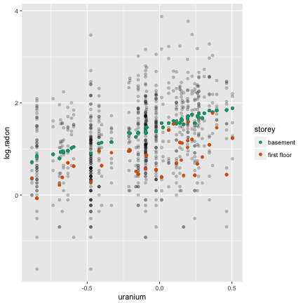
Plot of response vs covariate. What do you see?
Here's what we see
- Vertical stripes: each county is represented by an average uranium value
- Weak linear association, lots of variation for houses within county
- Four points inline horizontally at the base (be suspicious)
- Some counties only have 2, 3 points
- Scales?
Pre-processing
- Counties with less than 4 observations removed
- Four flat-line observations removed, really suspect these were erroneously coded missing values
Look again
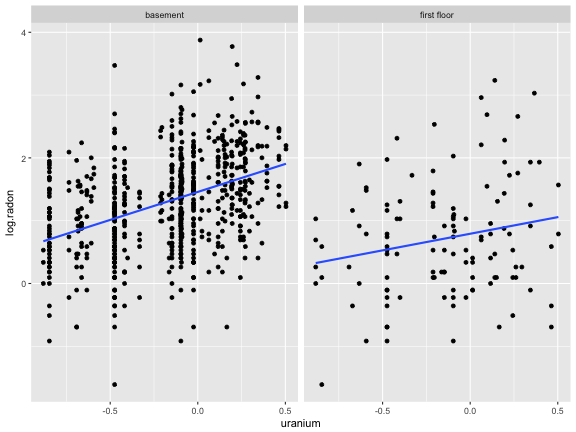
Fit a simple model
log.radon=β0+β1storey+β2uranium+ε
## ## Call:## glm(formula = log.radon ~ storey + uranium, data = radon_sub)## ## Deviance Residuals: ## Min 1Q Median 3Q Max ## -2.6610 -0.4928 0.0191 0.4745 2.4205 ## ## Coefficients:## Estimate Std. Error t value Pr(>|t|) ## (Intercept) 1.4483 0.0313 46.25 < 2e-16 ***## storeyfirst floor -0.6112 0.0733 -8.34 3.3e-16 ***## uranium 0.8359 0.0742 11.26 < 2e-16 ***## ---## Signif. codes: 0 '***' 0.001 '**' 0.01 '*' 0.05 '.' 0.1 ' ' 1## ## (Dispersion parameter for gaussian family taken to be 0.547)## ## Null deviance: 538.51 on 795 degrees of freedom## Residual deviance: 434.02 on 793 degrees of freedom## AIC: 1784## ## Number of Fisher Scoring iterations: 2Your turn
- What is the intercept?
- What is the slope?
- What does the coefficient labelled
storeyfirst floormean? - Make a sketch of what this model looks like.
- Does the model match the pattern observed in the data?
Fit an interaction term
## ## Call:## glm(formula = log.radon ~ storey * uranium, data = radon_sub)## ## Deviance Residuals: ## Min 1Q Median 3Q Max ## -2.6445 -0.4898 0.0131 0.4653 2.4369 ## ## Coefficients:## Estimate Std. Error t value Pr(>|t|) ## (Intercept) 1.4580 0.0318 45.91 < 2e-16 ***## storeyfirst floor -0.6659 0.0796 -8.37 2.7e-16 ***## uranium 0.8909 0.0805 11.07 < 2e-16 ***## storeyfirst floor:uranium -0.3620 0.2066 -1.75 0.08 . ## ---## Signif. codes: 0 '***' 0.001 '**' 0.01 '*' 0.05 '.' 0.1 ' ' 1## ## (Dispersion parameter for gaussian family taken to be 0.546)## ## Null deviance: 538.51 on 795 degrees of freedom## Residual deviance: 432.34 on 792 degrees of freedom## AIC: 1783## ## Number of Fisher Scoring iterations: 2What does this model look like?
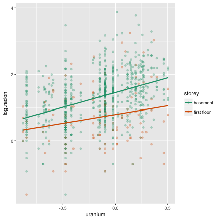
Your turn
Write down the equation of the fitted model.
Your turn
Write down the equation of the fitted model.
If story is basement, then
^y= 1.458 + 0.891 × uranium
and if story is first floor, then
^y= 0.792 + 0.529 × uranium
Mixed effects model
log.radonij=β0+β1storeyij+β2uraniumi+b0i+b1istoreyij+εij
i=1,...,#counties;j=1,...,ni
library(lme4)radon_lmer <- lmer(log.radon ~ storey + uranium + (storey | county.name), data = radon_sub)summary(radon_lmer)radon_lmer_fit <- augment(radon_lmer)Your turn
For the radon data:
- What is
p(number of fixed effects),q(number of random effects),g(number of groups)? - And hence
ni,i=1,…,g?
log.radonij=β0+β1storeyij+β2uraniumi+b0i+b1istoreyij+εij
i=1,...,#counties;j=1,...,ni
Examining the model output: fixed effects
Fixed effects: Estimate Std. Error t value(Intercept) 1.48066 0.03856 38.40storeyfirst floor -0.59011 0.11246 -5.25uranium 0.84600 0.09532 8.88How do these compare with the simple linear model estimates?
Coefficients: Estimate Std. Error t value Pr(>|t|) (Intercept) 1.44830 0.03131 46.254 < 2e-16 ***storeyfirst floor -0.61125 0.07332 -8.337 3.35e-16 ***uranium 0.83591 0.07422 11.262 < 2e-16 ***---Signif. codes: 0 ‘***’ 0.001 ‘**’ 0.01 ‘*’ 0.05 ‘.’ 0.1 ‘ ’ 1Examining the model output: random effects
Random effects: Groups Name Variance Std.Dev. Corr county.name (Intercept) 0.01388 0.1178 storeyfirst floor 0.22941 0.4790 0.02 Residual 0.50694 0.7120 Number of obs: 796, groups: county.name, 46This is saying that the variance of the estimates for first floor observations is larger than the storey.
What it looks like
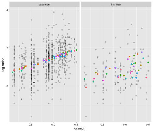
Or like this
Your turn
How does the mixed effects model differ from the simple linear model? (Hint: Think about the variance.)

Assumptions
Recall:
yi(ni×1)=Xi(ni×p)β(p×1)+Zi(ni×q)bi(q×1)+εi(ni×1)
biis a random sample fromN(0,D)and independent from the level-1 error terms,εifollow aN(0,σ2Ri)distributionDis a positive-definiteq×qcovariance matrix andRiis a positive-definiteni×nicovariance matrix
Extract and examine level-1 residuals
εi∼N(0,σ2Ri)
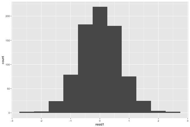
Level-1 (observation level) look normal.
QQ-plot
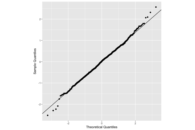
Level-1 (observation level) do look nearly normal.
Examine within group
Summary statistics
## # A tibble: 20 x 4## county.name m s n## <fctr> <dbl> <dbl> <int>## 1 ANOKA 0.05096 0.719 52## 2 BELTRAMI 0.33508 0.867 7## 3 BLUE EARTH 0.15188 0.562 14## 4 CARLTON -0.19433 0.651 10## 5 CARVER 0.32231 0.924 5## 6 CASS 0.38263 0.504 5## 7 CHISAGO 0.15472 0.845 6## 8 CLAY 0.16252 0.885 14## 9 CROW WING 0.04541 0.679 12## 10 DAKOTA -0.04153 0.717 63## 11 DOUGLAS 0.07803 0.329 9## 12 FARIBAULT -0.42081 0.311 5## 13 FREEBORN 0.31357 0.723 9## 14 GOODHUE 0.15537 0.719 14## 15 HENNEPIN -0.00737 0.662 105## 16 HOUSTON -0.13553 0.483 6## 17 HUBBARD -0.02903 0.712 5## 18 ITASCA 0.00484 0.584 11## 19 JACKSON 0.24493 0.689 5## 20 KOOCHICHING -0.10696 0.466 7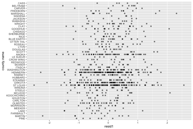
Learn
There is some difference on average between counties, which means that residuals still have some structure related to the county location.
Normality tests
Anderson-Darling, Cramer-von Mises, Lilliefors (Kolmogorov-Smirnov)
## ## Anderson-Darling normality test## ## data: radon_lmer_fit$resid1## A = 0.4, p-value = 0.4all believe that the residuals are consistent with normality.
Conclusion about level-1 residuals
The assumption:
εi∼N(0,σ2Ri)
is probably ok, at the worst it is not badly violated.
Random effects
bi∼N(0,D), i=1,…g
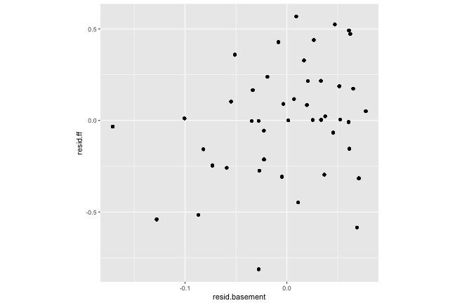
where D allows for correlation between random effects within group, and these should be independent from the level-1 error
We have both intercepts (basement) and slopes (first floor)
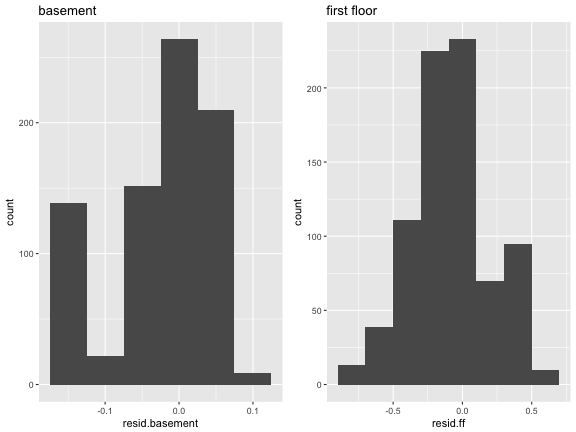
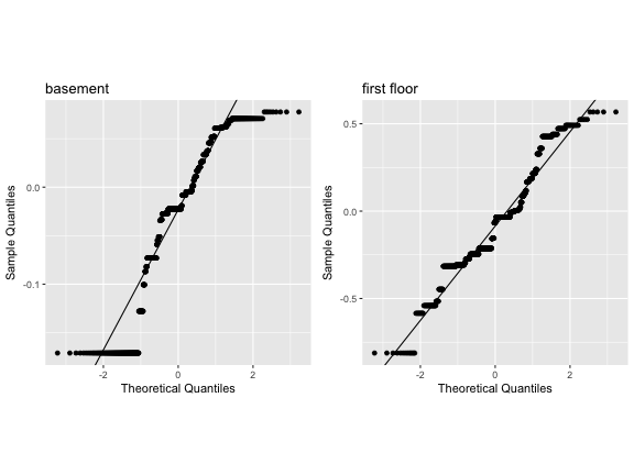
Should be no correlation
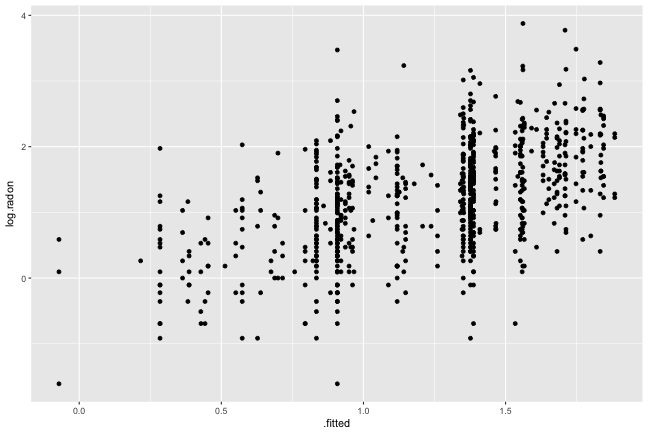
Fitted vs Observed
Plotting the observed vs fitted values, gives a sense for how much of the response is explained by the model. Here we can see that there is still a lot of unexplained variation.
Goodness of fit
From the linear model
## null.deviance df.null logLik AIC BIC deviance df.residual## 1 539 795 -887 1783 1806 432 792From the random effects model
## sigma logLik AIC BIC deviance df.residual## 1 0.712 -885 1784 1817 1760 789Hmmm... deviance looks strange! Compute sum of squares of residuals instead:
## [1] 387Which model is best?
Influence
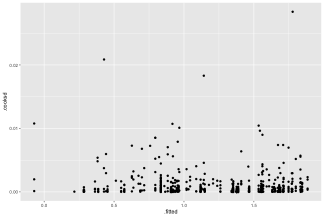
No overly influential observations
Share and share alike

This work is licensed under a Creative Commons Attribution 4.0 International License.